Compilation Process

The complete SiliconCompiler compilation is handled by a single call to the run() function. Within that function call, a static data flowgraph, consisting of nodes and edges is traversed and “executed.”

The static flowgraph approach was chosen for a number reasons:

• Performance scalability (“cloud-scale”)

• High abstraction level (not locked into one language and/or shared memory model)

• Deterministic execution

• Ease of implementation (synchronization is hard)

The Flowgraph

Nodes and Edges

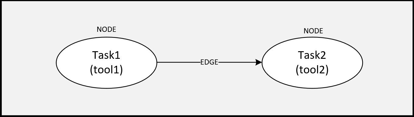
A SiliconCompiler flowgraph consists of a set of connected nodes and edges, where:

• A node is an executable tool performing some (”task”), and

• An edge is the connection between those tasks, specifying execution order.

Tasks

SiliconCompiler breaks down a “task” into an atomic combination of a step and an index, where:

1. A step is defined as discrete function performed within compilation flow such as synthesis, linting, placement, routing, etc, and

2. An index is defined as variant of a step operating on identical data.

An example of this might be two parallel synthesis runs with different settings after an import task. The two synthesis “tasks” might be called syn0 and syn1, where:

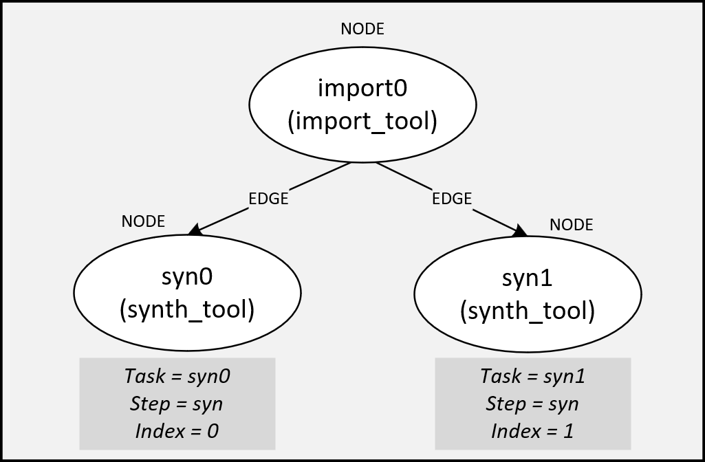
See Using Index for Optimization for more information on why using indices to build your flowgraph are helpful.

Execution

Flowgraph execution is done through the run() function which checks the flowgraph for correctness and then executes all tasks in the flowgraph from start to finish.

Flowgraph Examples

The flowgraph, used in the ASIC Demo, is a built-in compilation flow, called asicflow. This compilation flow is a pre-defined flowgraph customized for an ASIC build flow, and is called through the load_target() function, which calls a pre-defined PDK module that uses the asicflow flowgraph.

You can design your own chip compilation build flows by easily creating custom flowgraphs through:

• node()/edge() methods

The user is free to construct a flowgraph by defining any reasonable combination of steps and indices based on available tools and PDKs.

A Two-Node Flowgraph

The example below shows a snippet which creates a simple two-step (import + synthesis) compilation pipeline.

Snippet from examples/heartbeat_flowgraph.py

flow = 'synflow'
chip.node(flow, 'import', parse)               # use surelog for import
chip.node(flow, 'syn', syn_asic)               # use yosys for synthesis
chip.edge(flow, 'import', 'syn')               # perform syn after import
chip.set('option', 'flow', flow)

At this point, you can visually examine your flowgraph by using write_flowgraph(). This function is very useful in debugging graph definitions.

chip.write_flowgraph("flowgraph.svg", landscape=True)

Note

[In Progress] Insert link to tutorial which has step-by-step instruction on how to set up this flow with libs and pdk through run and execution.

Using Index for Optimization

The previous example did not include any mention of index, so the index defaults to 0.

While not essential to basic execution, the ‘index’ is fundamental to searching and optimizing tool and design options.

One example use case for the index feature would be to run a design through synthesis with a range of settings and then selecting the optimal settings based on power, performance, and area. The snippet below shows how a massively parallel optimization flow can be programmed using the SiliconCompiler Python API.

Snippet from examples/flowgraph_doe.py that sets up parallel synthesis runs for optimization

syn_strategies = ['DELAY0', 'DELAY1', 'DELAY2', 'DELAY3', 'AREA0', 'AREA1', 'AREA2']

# define flowgraph name
flow = 'synparallel'

# create import node
chip.node(flow, 'import', parse)

# create node for each syn strategy (first node called import and last node called synmin)
# and connect all synth nodes to both the first node and last node
for index in range(len(syn_strategies)):
    chip.node(flow, 'syn', syn_asic, index=str(index))
    chip.edge(flow, 'import', 'syn', head_index=str(index))
    chip.edge(flow, 'syn', 'synmin', tail_index=str(index))
    chip.set('tool', 'yosys', 'task', 'syn_asic', 'var', 'strategy', syn_strategies[index],
             step='syn', index=index)

    # set synthesis metrics that you want to optimize for
    for metric in ('cellarea', 'peakpower', 'standbypower'):
        chip.set('flowgraph', flow, 'syn', str(index), 'weight', metric, 1.0)

# create node for optimized (or minimum in this case) metric
chip.node(flow, 'synmin', minimum)

chip.set('option', 'flow', flow)

Note

[In Progress] Provide pointer to a tutorial on optimizing a metric